Morphometrics and the Procrustes analysis
Introduction
According to the Greek mythology, Procrustes was a highwayman who would invite anyone passing by his house to have a rest in a very special bed.
However, once a guest was lying on this particular bed, Procrustes would either stretch or chop off the guest’s limbs until this person matched the bed (and eventually died…). Luckily, the Greek hero Theseus captured Procrustes and killed him, by forcing him to fit his own unique bed.
This introduction and anything related to Procrustes sounds a bit scary now, so… why are we now using this name to analyse biological data in computational biology? Do not worry, this time nobody is hurt!! :)
When it comes to analyse biological data and we have information regarding different species, some of the questions we might first ask ourselves are “How closely related these species are?” or “When did they diverge from each other and how fast?”. The approaches that we can follow to answer them are different depending on the data we have.
Molecular data
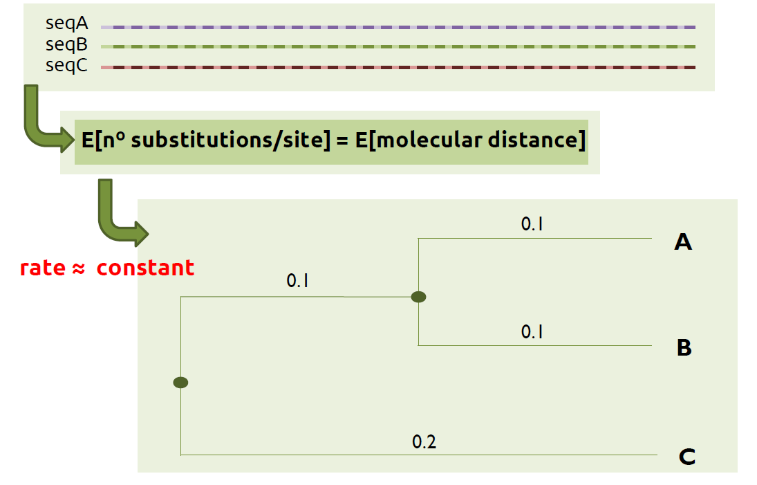
If we are working with molecular data, for instance nucleotide sequences, our first task can be to compute a molecular alignment so we can have a molecular tree that helps us to answer the previous questions.
Nowadays, various bioinformatics tools can be used for this purpose. In short and giving few details, they do the following:
- Measure pairwise distances: each pair of sequences is compared and the number of substitutions per site is calculated. This results into the molecular distances for each pair of species, also considered as estimates of the branch lengths.
- Return a molecular tree: a path that connects all the distances previously calculated is found, which results into the molecular tree.
If you want to generate a molecular tree, two of the most used softwares in evolutionary biology are the following:
- RAxML
This is a command-line tool with multiple options to generate your phylogenetic trees. It has a very detailed documentation with various examples for every option and, if you have still any doubt, you might want to visit their google group where your question might have been previously answered. Otherwise, they will try to help you as soon as possible! - BEAST2
This package contains different programs, although the ones that are of interest to generate a phylogenetic tree are the BEAUti2 and the BEAST2. The former is a java executable with a very user-friendly graphical interface that is used to prepare the input files to be used by BEAST2. Once this file inXMLformat is ready, BEAST2 can be used. Note that this tool is an executable file in Windows while it is launched through the terminal in Linux distributions. In order to get familiar with both tools, you can follow the tutorial Divergence Dating available in their website.
If you want to visualize the tree, you can use either FigTree or Dendroscope.
Morphological data
In contrast to molecular data, generating a morphological tree is not as straightforward as generating a molecular tree.
First of all, we need to have the same bones for all the species of the phylogeny. In other words, if we had a canine tooth for one of the species, we would need to have a canine tooth for the rest of the species. Otherwise, another bone that could be found for all the species (and in good conditions!) should be used for the morphological alignment. Afterwards, we need to get some landmark points from the bones that will be later used for the morphological alignment.
In morphometrics, we can distinguish three different types of landmarks:
- Anatomical landmarks: they are used to elucidate homologous regions between species.
- Mathematical landmarks: an algorithm determines where the landmark points should be according to a mathematical equation or specific geometrical function.
- Pseudo-landmarks: they are a combination of anatomical and mathematical landmarks.
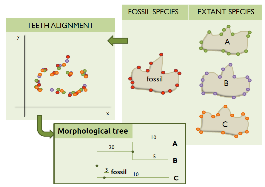
Let’s assume that we have managed to find the same teeth of three different extant species and also the same teeth of one fossil species. In this case, we will first need to scan the bones (i.e. digitalize them) and then use one of the available visualization tools to restore the images (i.e. possible cracks, breaks, or holes that might occur after the fossilization, excavation, or preparation techniques) and get the landmarks. If you are interested in how this procedure takes place, you can take a look at this post published by Emma Sherratt in which she clearly describes step by step different ways about how to gather both 2D and 3D landmarks.
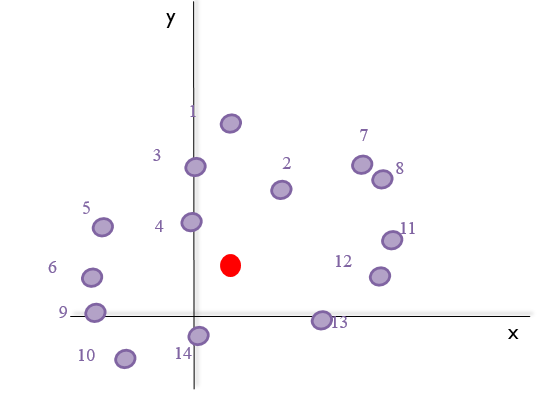
One might think that, after this tedious process, the algorithm to compute the morphological tree will simply have to superimpose the landmarks collected, calculate the distances, and then generate the tree; as this image shows:
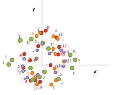
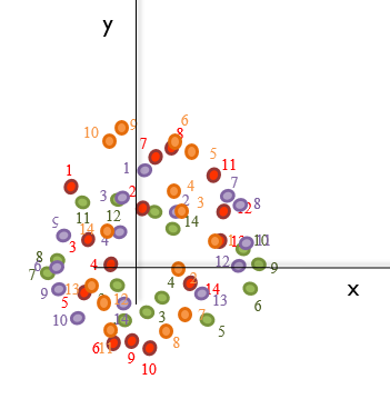
Unluckily, this is not always that easy as the bones do not tend to be oriented in the same direction during the scanning and/or collection of the landmarks. Therefore, if the landmarks collected were to be plotted, something like this is what computational biologists usually have to deal with:
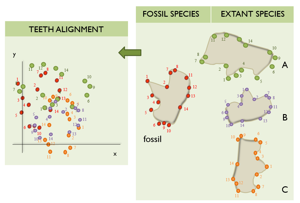
Note that these example plots are in 2D for simplicity, but the landmarks could have been collected in 3D.
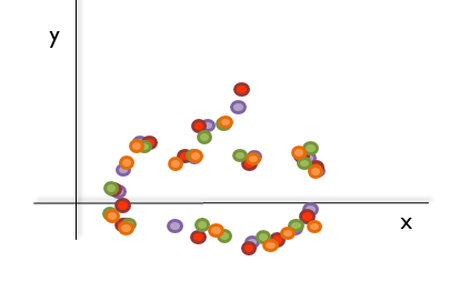
Consequently, these data have to be scaled to the same size so we can actually perform a proper alignment.
Oh wait… we are SCALING the data to the SAME SIZE… We are doing something similar to what Procrustes did to his guests, although we do not cause the data to suffer :) This similarity of fitting a shape into a specific size is the reason of naming this superimposition of landmark points as Procrustes analysis (PA).
However, it is important to note that you might find other terms in the literature being used to describe this same concept:
- Procrustes superimposition (PS)
- Procrustes fitting (PF)
- Generalized Procrustes Analysis (GPA)
- Generalized least squares (GLS)
- Least squares fitting (LSF)
Particularly, the algorithm that performs the PA carries out the following tasks:
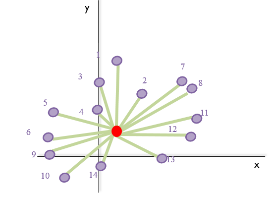
- It centers all the specimens to the origin, i.e. in 2D they are centered to \(\mathrm{P}(x=0,y=0)\) and in 3D to \(\mathrm{P}(x=0,y=0,z=0)\).
- It calculates the mean of the landmark points, the centroid. For instance, for the shape of species B (purple), this would be:
- It sums all the distances from the centroid to each landmark (green arrows in the image below), the centroid size. Taking the previous image into account:
- It scales every specimen to unit-centroid size (size = 1.0).
- It rotates them around the origin until the coordinates of the corresponding landmark points are as close as
possible. In other words, it minimizes the sum of squared distances among the coordinates.
Note that the images above are just informative and basically aim to help to understand the concept of the PA. The landmarks have not been collected from any data set nor follow any specific pattern. One should not take any possible error when placing the landmarks or rotating the shapes into account as these figures are only representations of this procedure.
Now that we understand the importance of the PA applied to the study of morphological data, let’s see how we can apply this theory to some data!
Procrustes analysis with R
The data set
In the previous section, we have seen how a morphological alignment could look like before and after performing a PA. However, how would a data set really look like?
Normally, the landmarks for all the specimens are collected and saved in a matrix, \(\mathrm{M}\). Each column will contain one coordinate. If the landmarks are 2D points, then every two columns we will have the coordinates for each point. For instance, if we have 10 landmark points, we will have 2 x 10 = 20 coordinates. Therefore, the first two columns (without taking into account possible extra columns containing information about the specimens) will refer to the first landmark, \(L_1=(x_1,y_1)\), the third and fourth columns to the second landmark, \(L_2=(x_2,y_2)\), and so on. Every \(i^{th}\) row in \(\mathrm{M}\) will then be the vector of the coordinates of all landmarks for specimen \(i\).
| Specimens | L1.x | L1.y | L2.x | L2.y | |
|---|---|---|---|---|---|
| Sp.1 | 0.123 | 0.456 | 0.150 | 0.320 | … |
| Sp.2 | -0.145 | -0.362 | -0.120 | -0.502 | … |
| … | |||||
According to this notation, the element \(\mathbf{m_{1,2}}\) would be the \(y\) coordinate of the first landmark taken from the first specimen. Now that we are familiar with the format of our data set, let’s start the practical!
Tutorial
1. Downloading the material
In order to start the practical, you will need to download the data that WE are going to be working with from my GitHub repository.
You can download it in zip format and save it in your preferred directory. However, if you want to use the terminal and have git installed, you can cd to the directory you want to save the data in your laptop and type the following:
git clone https://github.com/sabifo4/Morphometrics_practical
You will see that there are three folders, an R script, and a README.md file. Let’s look at each of them:
- The
datafolder contains the data that you are going to analyse: the file “Triturus_and_Calotriton_lmk_reduced.csv”. This contains 48 3D landmarks collected from the skulls of 8 Triturius specimens and 1 Calotriton specimen (see Ivanović A, Arntzen JW for more information). - The
PAfolder contains two files, each of them being an example of the results you should get after performing the PA while following this tutorial. - The
plotsfolder contains three plots, the ones you should get while going through this tutorial. - The R script
Morphometrics_practical.Rcontains all the commands that we are going to go through in this tutorial and explain them step by step. - The
README.mdfile is just a description of what the repository contains.
2. Starting R: aetting the working environment
Now, please start R or RStudio, the one you feel more comfortable working with. We will first clean the environment and load the packages we will need:
#\\ Clean environment
rm(list=ls())

#\\ Load needed packages
library(maptools)
library(geomorph)
If you do not have these packages installed, please install them by running the following commands:
#\\ Install geomorph
install.packages("geomorph")

#\\ Install maptools
install.packages("maptools")
Now, let’s set your working environment so R can know where the data set that you have downloaded is. You can do this in two ways:
- If you know the absolute path to your directory, you can type the following:
#\\ Get the path to your directory
wd <- "path_your_directory/"

#\\ Set the working directory
setwd(wd)
- If you do not know excatly the absolute path to your directory and/or is so long that you do not want to type it, let’s tell R to ask you for the location of the file so we can later get the absolute path:
#\\ Type the name of the R script
filename <- "Morphometrics_practical.R"

#\\ Let's ask R to open a window so we can navigate
#\\ through our laptop and find the R script
filepath <- file.choose()  # browse and select your_file.R in the window

#\\ Let's get the string that contains only the path to the directory
#\\ ommitting the name of the R script
wd = substr(filepath, 1, nchar(filepath)-nchar(filename))

#\\ If you are using Windows, you should run the following command
wd <- gsub(pattern="[\\]", replace="/", x=wd)

#\\ Set working directory
setwd(wd)
3. Create variables
Now that R knows where your directory is, let’s load the data set we are going to be working with and save it in the data.frame object df:
#\\ Load data set - 9 species x (3 info columns + 144 coordinates)
df <- read.table(file=paste(wd,"data/Triturus_and_Calotriton_lmk_reduced.csv", sep=""),
                 header=T,sep=",", dec=".", stringsAsFactors=F)
If you open this file with your favourite text editor (e.g. Notepad++, sublime, atom, …), you will see that there are 3 extra columns
(Voucher number, Species, NRBV) with some information about the specimens which landmarks have been collected from:
Voucher number	Species			NRBV	x1		x2
nl44640 	Calotriton asper	14	-0.005383228	-2.91E-04
9107_783 	Triturus carnifex	14	0.004734634	0.001809802
251		Triturus cristatus	15	-0.001610397	0.001812907
11c10 		Triturus dobrogicus	16	0.001972431	-0.003228118
22885		Triturus ivanbureschi	13	-0.005712633	-3.05E-04
22242		Triturus karelinii	13	-0.006407888	6.87E-04
12c30 		Triturus macedonicus	14	-0.001910315	0.00405883
9074m467 	Triturus marmoratus	12	0.00237951	0.003246724
7615 73		Triturus pygmaeus	12	-0.002393209	-0.002001612
In order to perform the PA, we do not need these columns. Therefore, we can get rid of them, although we can keep the names of the specimens (\(2^{nd}\) column) as row names:
#\\ The first 3 columns do not contain the coordinates
#\\ Get from the 4th to the nth column, where the data is
mm <- df[,4:(dim(df)[2])] # 9sp x 144coords (144/3=48 lmk)

#\\ Get name of specimens as row names
rownames(mm) <- df[,2]
We have now loaded our data and filtered it to have only the coordinates. However, we still do not have the correct format required by geomorph::gpagen. Specifically, this function needs the data to be in an array format. As our data contains 3D landmarks, we will need a tridimensional array. The dimensions of the array are \(p\) \(\mathrm{x}\) \(k\) \(\mathrm{x}\) \(n\), being \(p\) the amount of coordinates \((p = 144)\), \(k\) the dimensions of the data set \((k = 3)\), and \(n\) the number of specimens \((n = 9)\).
In order to create this array, we first have to define its imensions. In order to name the variables that will contain the dimensions of this array, we are going to use names that help us to remember what our variables are:
- We name the variable to store the \(p\) coordinates as
num.coords. - We name the variable to save the \(k\) dimensions of the data as
coor3D. - We name the variable to save the \(n\) specimens as
ns.
#\\ Set variables to define the dimensions of the 3D array
num.coords <- dim(mm)[2]
coor3D <- 3
ns <- 9

#\\ Create an empty array to store the coordinates in the format
#\\ p x k x n (num.coords x coor3D x ns)
ma <- array(dim=c(num.coords/coor3D, coor3D, ns)) # 48 lmks, 3D, 9 specimens
Now we have our empty array in the format that geomorph::gpagen needs. In order to fill it in with the coordinates, we first need to define which columns from our data.frame mm are \(x\) coordinates, \(y\) coordinates, and \(z\) coordinates:
#\\ Select the positions from 1 to 144 that correspond to
#\\ x coords, y coords, and z coords
xi <- seq(from=1, to=num.coords, by=coor3D); yi <- xi+1; zi <- yi+1
4. Prepare the data set in array format
In the previous step, we created an empty 3D array with dimensions \(p = 144\) (number of coordinates), \(k = 3\) (dimensions of the data set), and \(n = 9\) (the number of specimens). Now it is time to fill it in with the data!
# Note that we need to first unlist the objects
# "mm[i,xi]", "mm[i,yi]", and "mm[i,zi]"
# because each coordinate belongs to one list of vectors
# from the data.frame "mm"
for (i in 1:ns) {
  ma[,1,i] <- unlist(mm[i,xi])
  ma[,2,i] <- unlist(mm[i,yi])
  ma[,3,i] <- unlist(mm[i,zi])
}
You might have noticed that we added the function unlist when we were getting the \(x\), \(y\), or \(z\) coordinates from the data.frame mm. This is because each coordinate belongs to one list of vectors in mm. For example, mm$astl is the column vector that contains all the \(x\) coordinates of the first landmark (one for each specimen), mm$$astl.1 the column vector with all the \(y\) coordinates of the first landmark, and so on. However, the coordinates of all landmarks for one specimen (what we do with the command mm[i,xi] in the for loop above) belong to different column vectors from which only one of the 9 elements (one coordinate per specimen) is the one we want to extract. You can see this if you type the following example:
#\\ Column vector of coordinates x for landmark 1
#\\ from which we get the first element (coordinate
#\\ x of first specimen)
mm$astl[1]

#\\ First coordinate, coordinate x, for landmark 1
#\\ collected from specimen 1
mm[1,1]

#\\ See if they are equal
all.equal(mm$astl[1], mm[1,1])
#[1] TRUE
According to this, we need to unlist these column vectors so we can get only the coordinates we are interested in for each specimen during the for loop. And that is what we did!
5. Run Procrustes analysis
We finally have our data set in the correct format, so we can run geomorph::gpagen! We will store the list of objects that this function returns in the object ma.paln so we can later work with the results of the PA:
#\\ Get procrustes analysis done
ma.paln <- geomorph::gpagen(ma)
CONGRATULATIONS!!! You have just carried out a Procrustes analysis!! :)
There are different objects in the list ma.paln, but we are mainly interested for this tutorial in the one that contains the scaled and optimally rotated coordinates after having performed the PA: the object coords.
As ma.paln is a list, we can access this object as ma.paln$coords. If we want to save these coordinates, we cannot save them in an array format, hence we have to convert them back to the format we previously had in the data.frame called mm: \(n\) rows (number of specimens) and \(p\) columns (number of coordinates). Therefore, we need to create an empty matrix (because now we want to input only numerical values, the coordinates) with these imensions that will later fill in with the resulting coordinates:
#\\ Create empty array with n=ns and p=num.coords
faln <- matrix(0, nrow=ns, ncol=num.coords)

#\\ Fill in the array with scaled and optimally rotated
#\\ coordinates
for (i in 1:ns) {
  faln[i,xi] <- ma.paln$coords[,1,i]
  faln[i,yi] <- ma.paln$coords[,2,i]
  faln[i,zi] <- ma.paln$coords[,3,i]
}
If we wanted, now we could save these coordinates in a csv file:
#\\ Save only coordinates
write.table(faln, file="PA/Triturus_and_Calotriton_after_PA_clean.csv",
             row.names=F, col.names=F, quote=F, sep=",")

#\\ Save coordinates + 3 columns of info about specimens
#\\ by appending these 3 columns from the first loaded data set 'df'
#\\ to the matrix with the resulting coordinates from PA, 'faln'
faln.rn <- cbind(df[,1:3], faln)
colnames(faln.rn) <- colnames(df)
write.table(faln.rn, file="PA/Triturus_and_Calotriton_after_PA.csv",
             row.names=F, quote=F, sep=",")
6. Plots
Last but not least, it is always nice to actually see what is going on behind the code we write, if we can. Plotting the data or generating an image can always help us to understand how the data are being processed by the algorithms we write in our code.
In this case, it is very interesting to compare the plot of the landmarks of each specimen before and after performing the PA. Thus, we can see how our data were harmlessly stretched or chopped off by the Procrustes algorithm in geomorph::gpagen :)
We can either plot the results in 3D or in 2D, although if you want to keep the plot you will have to keep the 2D plots. If you run the following code, it will result in three 2D plots:
- The first plot will be the alignment of the landmarks before performing the PA.
- The second plot will be the alignment of the landmarks after performing the PA.
- The third plot is like the first one but with the lines x=0 and y=0 added.
The function maptools::pointLabel is commented, although you can
uncommented if you want to see in your plot the number of each landmark per
specimen plotted. Depending on the specimen’s landmarks which landmark number you
want to see, you might modify the code.
#\\ Plot the data set before PA
#
# Uncomment the two commented lines if you want to save
# this plot
#
# pdf("plots/Raw_data_2D.pdf", paper="a4", width=15, height=15)
plotAllSpecimens(ma[,1:2,])
# dev.off()

#\\ Plot the data set after PA
# Uncomment the two commented lines if you want to save
# this plot
#
# pdf("plots/Data_after_PA_2D.pdf", paper="a4", width=15, height=15)
plotAllSpecimens(ma.paln$coords[,1:2,])
# dev.off()

#\\ Plot a 2D procrustes plot with lines x=0 and y=0 and mean shape
#
# Here we have decided to add to the plot the mean of every group of
# landmarks (one landmark per specimen) that fall to the same point
# in the plot forming the skull shape --> "points()"
#
# If you want to plot the labels of the landmarks of the 1st
# and the 2nd specimen, just uncomment the command that calls the function
# "maptools::pointLabel". You can change the numbers if you want to see
# other landmarks or you can also leave this uncommented
#
# NOTE: Uncomment the lines with "pdf()" and "dev.off()" if you want to save
#       this plot
#
#pdf("plots/Data_after_PA_2D_limits.pdf", paper="a4", width=15, height=15)
msh <- mshape(ma.paln$coords[,1:2,])
xl <- range(faln[,xi]); yl <- range(faln[,yi])
matplot(faln[1:ns,xi], faln[1:ns,yi], pch='+', cex=.5, asp=1, col="darkgrey", xlim=xl, ylim=yl, xlab="X", ylab="Y", las=1)
points(msh[,1], msh[,2],cex=1, pch=19,col="black")
# maptools::pointLabel(faln[1:2,xi], faln[1:2,yi], labels = paste(1:dim(msh)[1]),cex=1,col=c("black", "red"),
#                      method = c("SANN"),
#                      allowSmallOverlap = FALSE,
#                      trace = FALSE,
#                      doPlot = TRUE
# )
abline(h=0, v=0, lty=2, lwd=.25)
#dev.off()
And here the tutorial comes to an end!
I hope you have found this tutorial useful and you have enjoyed learning about the Procrustes analysis and its application to morphometrics!
References
- Felsenstein, Joseph, Inferring phylogenies (Sinauer Associates, 2004).
- Ivanović A, Arntzen JW (2014) The evolution of skull and body shape in Triturus newts reconstructed from 3D morphometric data and phylogeny. Biological Journal of the Linnean Society 113(1): 243-255.
- Ivanović A, Arntzen JW (2014) Data from: The evolution of skull and body shape in Triturus newts reconstructed from 3D morphometric data and phylogeny. Dryad Digital Repository.
- Adams, D. C., M. L. Collyer, A. Kaliontzopoulou, and E. Sherratt. (2017). Geomorph: Software for geometric morphometric analyses. R package version 3.0.5.
- Roger Bivand and Nicholas Lewin-Koh (2017). maptools: Tools for Reading and Handling Spatial Objects. R package version 0.9-2.